DSSC detector geometry

As of version 0.5, karabo_data has geometry code for the DSSC detector. This doesn’t currently account for the hexagonal pixels of DSSC, but it’s good enough for a preview of detector images.

%matplotlib inline
from karabo_data.geometry2 import DSSC_1MGeometry

# Made up numbers!
quad_pos = [
    (-130, 5),
    (-130, -125),
    (5, -125),
    (5, 5),
]
path = 'dssc_geo_june19.h5'

g = DSSC_1MGeometry.from_h5_file_and_quad_positions(path, quad_pos)

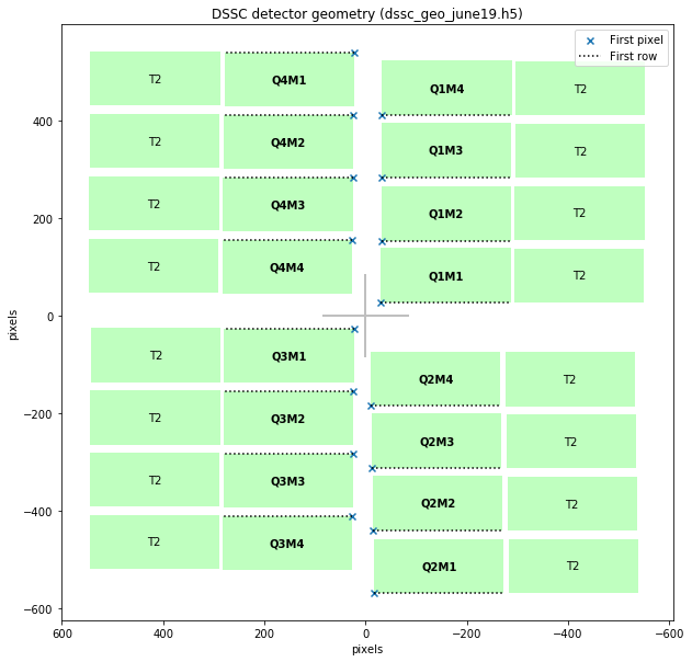
g.inspect()

<matplotlib.axes._subplots.AxesSubplot at 0x2ac10f8709b0>

import numpy as np
import matplotlib.pyplot as plt

g.expected_data_shape

(16, 128, 512)

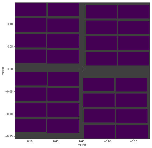
We’ll use some empty data to demonstate assembling an image.

a = np.zeros(g.expected_data_shape)

g.plot_data_fast(a, axis_units='m');

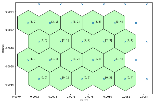
Let’s have a close up look at some pixels in Q1M1. get_pixel_positions() gives us pixel centres. to_distortion_array() gives pixel corners in a slightly different format, suitable for PyFAI.

PyFAI requires non-negative x and y coordinates. But we want to plot them along with the centre positions, so we pass allow_negative_xy=True to get comparable coordinates.

pixel_pos = g.get_pixel_positions()
print("Pixel positions array shape:", pixel_pos.shape,
      "= (modules, slow_scan, fast_scan, x/y/z)")
q1m1_centres = pixel_pos[0]
cx = q1m1_centres[..., 0]
cy = q1m1_centres[..., 1]

distortn = g.to_distortion_array(allow_negative_xy=True)
print("Distortion array shape:", distortn.shape,
      "= (modules * slow_scan, fast_scan, corners, z/y/x)")
q1m1_corners = distortn[:128]

Pixel positions array shape: (16, 128, 512, 3) = (modules, slow_scan, fast_scan, x/y/z)
Distortion array shape: (2048, 512, 6, 3) = (modules * slow_scan, fast_scan, corners, z/y/x)

from matplotlib.patches import Polygon
from matplotlib.collections import PatchCollection

fig, ax = plt.subplots(figsize=(10, 10))

hexes = []
for ss_pxl in range(4):
    for fs_pxl in range(5):

        # Create hexagon
        corners = q1m1_corners[ss_pxl, fs_pxl]
        corners = corners[:, 1:][:, ::-1]  # Drop z, flip x & y
        hexes.append(Polygon(corners))

        # Draw text label near the pixel centre
        ax.text(cx[ss_pxl, fs_pxl], cy[ss_pxl, fs_pxl],
                '  [{}, {}]'.format(ss_pxl, fs_pxl),
                verticalalignment='bottom', horizontalalignment='left')

# Add the hexagons to the plot
pc = PatchCollection(hexes, facecolor=(0.75, 1.0, 0.75), edgecolor='k')
ax.add_collection(pc)

# Plot the pixel centres
ax.scatter(cx[:5, :6], cy[:5, :6], marker='x')

# matplotlib is reluctant to show such a small area, so we need to set the limits manually
ax.set_xlim(-0.007, -0.0085)  # To match the convention elsewhere, draw x right-to-left
ax.set_ylim(0.0065, 0.0075)
ax.set_ylabel("metres")
ax.set_xlabel("metres")
ax.set_aspect(1)