Detector geometry for AGIPD
The AGIPD detector, which is already in use at the SPB experiment, consists of 16 modules of 512×128 pixels each. Each module is further divided into 8 ASICs.
To view or analyse detector data, we need to apply geometry to find the positions of pixels.
[1]:
%matplotlib inline
import matplotlib.pyplot as plt
import numpy as np

from karabo_data import RunDirectory, stack_detector_data
from karabo_data.geometry2 import AGIPD_1MGeometry
Fetch AGIPD detector data for one pulse to test with:
[2]:
run = RunDirectory('/gpfs/exfel/exp/SPB/201831/p900039/proc/r0273/')
[3]:
tid, train_data = run.select('*/DET/*', 'image.data').train_from_index(60)
[4]:
stacked = stack_detector_data(train_data, 'image.data')
stacked_pulse = stacked[10]
stacked_pulse.shape
[4]:
(16, 512, 128)
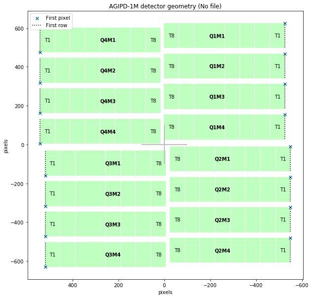
Generate a simple geometry given the (x, y) coordinates of the first pixel in the first module of each quadrant, in pixel units relative to the centre, where the beam passes through the detector.
There are also methods to load and save CrystFEL format geometry files.
[5]:
geom = AGIPD_1MGeometry.from_quad_positions(quad_pos=[
        (-525, 625),
        (-550, -10),
        (520, -160),
        (542.5, 475),
    ])
[6]:
geom.inspect()
[6]:
<matplotlib.axes._subplots.AxesSubplot at 0x2b1dae4100f0>
The pixels are not necessarily all aligned, so precisely assembling data in a 2D array requires interpolation, which is slow:
[7]:
%%time
data, centre_yx = geom.position_modules_interpolate(stacked_pulse)
print(data.shape)
(1258, 1094)
CPU times: user 10.9 s, sys: 1.08 s, total: 11.9 s
Wall time: 6 s
But we know that the modules are closely aligned with the axes, so we can ‘snap’ the geometry to the grid and copy data more efficiently:
[8]:
%%time
data, centre_yx = geom.position_modules_fast(stacked_pulse)
print(data.shape)
(1256, 1092)
CPU times: user 23.9 ms, sys: 9.73 ms, total: 33.6 ms
Wall time: 29.6 ms
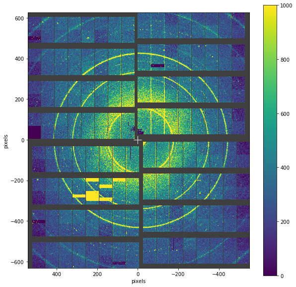
Plot the detector image
Data can be directly plotted using the plot_data_fast method.
[9]:
geom.plot_data_fast(stacked_pulse, vmin=0, vmax=1000)
[9]:
<matplotlib.axes._subplots.AxesSubplot at 0x2b1e67f828d0>
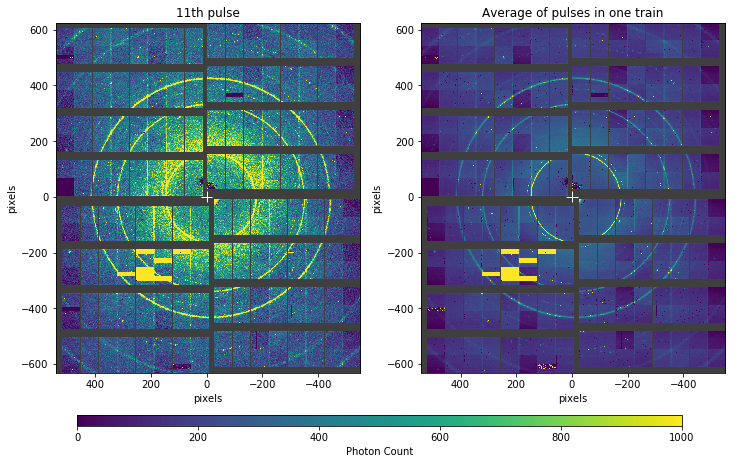
You can control the plot using keyword arguments for axis and colorbar. For example, to plot two images in the same figure:
[10]:
fig, (ax0, ax1) = plt.subplots(ncols=2, figsize=(12, 7.5))
ax_cbar = fig.add_axes([0.15, 0.08, 0.7, 0.02])  # Create extra axes for the colorbar

# Plot a single pulse in the left axes
geom.plot_data_fast(stacked_pulse, vmin=0, vmax=1000, ax=ax0, colorbar={
                        'cax': ax_cbar,
                        'shrink': 0.6,
                        'pad': 0.1,
                        'orientation': 'horizontal'
                    })
ax0.set_title('11th pulse')

# Label the colorbar associated with the first image
colorbar = ax0.images[0].colorbar
colorbar.set_label('Photon Count')

# Plot the average over all pulses on the right.
# Disable the colorbar because it's the same scale as the left image.
geom.plot_data_fast(stacked.mean(axis=0), vmin=0, vmax=1000, ax=ax1, colorbar=False)
ax1.set_title('Average of pulses in one train')
[10]:
Text(0.5, 1.0, 'Average of pulses in one train')
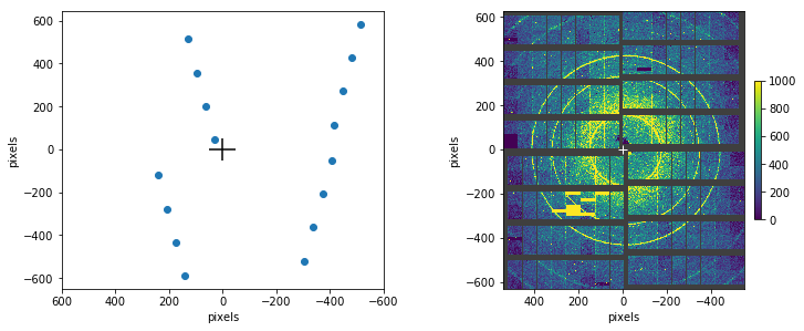
Converting array positions to physical positions
We can also convert array coordinates within the detector data into real (x, y, z) positions in metres.
[11]:
# Generate some array coordinates, one in each module
module_no = np.arange(0, 16)
# For AGIPD, slow-scan is the x dimension, increasing from the edges towards the centre
slow_scan = np.linspace(10, 500, num=16)
fast_scan = np.full(fill_value=40.1, shape=16)  # Fixed y position in each module
[12]:
positions = geom.data_coords_to_positions(module_no, slow_scan, fast_scan)
print("positions.shape =", positions.shape)  # (point, x/y/z)

# Convert metres to pixel units to compare with plots above
px = positions[:, 0] / geom.pixel_size
py = positions[:, 1] / geom.pixel_size

fig, (ax0, ax1) = plt.subplots(1, 2, figsize=(12, 6))

ax0.scatter(px, py)
ax0.set_xlabel('pixels')
ax0.set_ylabel('pixels')
ax0.hlines(0, -50, 50)  # Draw a cross at the origin
ax0.vlines(0, -50, 50)  #
ax0.set_xlim(600, -600)  # Invert x-axis to match plots above

# Display the image alongside it for comparison
geom.plot_data_fast(stacked_pulse, vmin=0, vmax=1000, ax=ax1,
                    colorbar={'shrink': 0.5, 'pad': 0.03})
fig.subplots_adjust(bottom=0.3, wspace=0.3)
positions.shape = (16, 3)