AGIPD, LPD & DSSC Geometry¶

The AGIPD and LPD detectors are made up of several sensor modules, from which separate streams of data are recorded. Inspecting or processing data from these detectors therefore depends on knowing how the modules are arranged. The module karabo_data.geometry2 handles this information.

All the coordinates used in this module are from the detector centre. This should be roughly where the beam passes through the detector. They follow the standard European XFEL axis orientations, with x increasing to the left (looking along the beam), and y increasing upwards.

Note

This module includes methods to assemble data into a single array. This is sufficient for a quick examination of detector images, but the detector pixels may not line up with the grid imposed by a single array. For accurate analysis, it’s best to use a tool that can process geometry internally with sub-pixel precision.

AGIPD-1M¶

AGIPD-1M consists of 16 modules of 512×128 pixels each. Each module is further subdivided into 8 tiles. The layout of tiles within a module is fixed by the manufacturing process, but this geometry code works with a position for each tile.

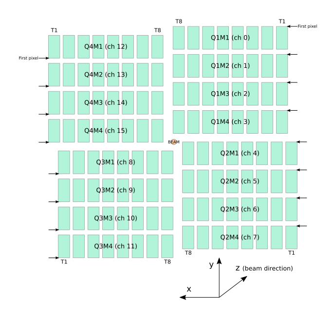
The approximate layout of AGIPD-1M, in a front view (looking along the beam).¶

class karabo_data.geometry2.AGIPD_1MGeometry(modules, filename='No file')¶

Detector layout for AGIPD-1M

The coordinates used in this class are 3D (x, y, z), and represent metres.

You won’t normally instantiate this class directly: use one of the constructor class methods to create or load a geometry.

classmethod from_quad_positions(quad_pos, asic_gap=2, panel_gap=29, unit=0.0002)¶

Generate an AGIPD-1M geometry from quadrant positions.

This produces an idealised geometry, assuming all modules are perfectly flat, aligned and equally spaced within their quadrant.

The quadrant positions are given in pixel units, referring to the first pixel of the first module in each quadrant, corresponding to data channels 0, 4, 8 and 12.

The origin of the coordinates is in the centre of the detector. Coordinates increase upwards and to the left (looking along the beam).

To give positions in units other than pixels, pass the unit parameter as the length of the unit in metres. E.g. unit=1e-3 means the coordinates are in millimetres.

classmethod from_crystfel_geom(filename)¶

Read a CrystFEL format (.geom) geometry file.

Returns a new geometry object.

write_crystfel_geom(filename, *, data_path='/entry_1/instrument_1/detector_1/data', mask_path=None, dims=('frame', 'modno', 'ss', 'fs'), adu_per_ev=None, clen=None, photon_energy=None)¶

Write this geometry to a CrystFEL format (.geom) geometry file.

Parameters

filename (str) – Filename of the geometry file to write.
data_path (str) – Path to the group that contains the data array in the hdf5 file. Default: '/entry_1/instrument_1/detector_1/data'.
mask_path (str) – Path to the group that contains the mask array in the hdf5 file.
dims (tuple) – Dimensions of the data. Extra dimensions, except for the defaults, should be added by their index, e.g. (‘frame’, ‘modno’, 0, ‘ss’, ‘fs’) for raw data. Default: ('frame', 'modno', 'ss', 'fs'). Note: the dimensions must contain frame, ss, fs.
adu_per_ev (float) – ADU (analog digital units) per electron volt for the considered detector.
clen (float) – Distance between sample and detector in meters
photon_energy (float) – Beam wave length in eV

get_pixel_positions(centre=True)¶

Get the physical coordinates of each pixel in the detector

The output is an array with shape like the data, with an extra dimension of length 3 to hold (x, y, z) coordinates. Coordinates are in metres.

If centre=True, the coordinates are calculated for the centre of each pixel. If not, the coordinates are for the first corner of the pixel (the one nearest the [0, 0] corner of the tile in data space).

to_distortion_array(allow_negative_xy=False)¶

Return distortion matrix for AGIPD detector, suitable for pyFAI.

Parameters

allow_negative_xy (bool) – If False (default), shift the origin so no x or y coordinates are negative. If True, the origin is the detector centre.

Returns

out – Array of float 32 with shape (8192, 128, 4, 3). The dimensions mean:

8192 = 16 modules * 512 pixels (slow scan axis)
128 pixels (fast scan axis)
4 corners of each pixel
3 numbers for z, y, x

Return type

ndarray

plot_data_fast(data, *, axis_units='px', frontview=True, ax=None, figsize=None, colorbar=True, **kwargs)¶

Plot data from the detector using this geometry.

This approximates the geometry to align all pixels to a 2D grid.

Returns a matplotlib axes object.

Parameters

data (ndarray) – Should have exactly 3 dimensions, for the modules, then the slow scan and fast scan pixel dimensions.
axis_units (str) – Show the detector scale in pixels (‘px’) or metres (‘m’).
frontview (bool) – If True (the default), x increases to the left, as if you were looking along the beam. False gives a ‘looking into the beam’ view.
ax (~matplotlib.axes.Axes object, optional) – Axes that will be used to draw the image. If None is given (default) a new axes object will be created.
figsize (tuple) – Size of the figure (width, height) in inches to be drawn (default: (10, 10))
colorbar (bool, dict) – Draw colobar with default values (if boolean is given). Colorbar appearance can be controlled by passing a dictionary of properties.
kwargs – Additional keyword arguments passed to ~matplotlib.imshow

position_modules_fast(data, out=None)¶

Assemble data from this detector according to where the pixels are.

This approximates the geometry to align all pixels to a 2D grid.

Parameters

data (ndarray) – The last three dimensions should match the modules, then the slow scan and fast scan pixel dimensions.
out (ndarray, optional) – An output array to assemble the image into. By default, a new array is allocated. Use output_array_for_position_fast() to create a suitable array. If an array is passed in, it must match the dtype of the data and the shape of the array that would have been allocated. Parts of the array not covered by detector tiles are not overwritten. In general, you can reuse an output array if you are assembling similar pulses or pulse trains with the same geometry.

Returns

out (ndarray) – Array with one dimension fewer than the input. The last two dimensions represent pixel y and x in the detector space.
centre (ndarray) – (y, x) pixel location of the detector centre in this geometry.

output_array_for_position_fast(extra_shape=(), dtype=<class 'numpy.float32'>)¶

Make an empty output array to use with position_modules_fast

You can speed up assembling images by reusing the same output array: call this once, and then pass the array as the out= parameter to position_modules_fast(). By default, it allocates a new array on each call, which can be slow.

Parameters

extra_shape (tuple, optional) – By default, a 2D output array is generated, to assemble a single detector image. If you are assembling multiple pulses at once, pass extra_shape=(nframes,) to get a 3D output array.
dtype (optional (Default: np.float32)) –

position_modules_interpolate(data)¶

Assemble data from this detector according to where the pixels are.

This performs interpolation, which is very slow. Use position_modules_fast() to get a pixel-aligned approximation of the geometry.

Parameters

data (ndarray) – The three dimensions should be channelno, pixel_ss, pixel_fs (lengths 16, 512, 128). ss/fs are slow-scan and fast-scan.

Returns

out (ndarray) – Array with the one dimension fewer than the input. The last two dimensions represent pixel y and x in the detector space.
centre (ndarray) – (y, x) pixel location of the detector centre in this geometry.

inspect(axis_units='px', frontview=True)¶

Plot the 2D layout of this detector geometry.

Returns a matplotlib Axes object.

Parameters

axis_units (str) – Show the detector scale in pixels (‘px’) or metres (‘m’).
frontview (bool) – If True (the default), x increases to the left, as if you were looking along the beam. False gives a ‘looking into the beam’ view.

compare(other, scale=1.0)¶

Show a comparison of this geometry with another in a 2D plot.

This shows the current geometry like inspect(), with the addition of arrows showing how each panel is shifted in the other geometry.

Parameters

other (AGIPD_1MGeometry) – A second geometry object to compare with this one.
scale (float) – Scale the arrows showing the difference in positions. This is useful to show small differences clearly.

data_coords_to_positions(module_no, slow_scan, fast_scan)¶

Convert data array coordinates to physical positions

Data array coordinates are how you might refer to a pixel in an array of detector data: module number, and indices in the slow-scan and fast-scan directions. But coordinates in the two pixel dimensions aren’t necessarily integers, e.g. if they refer to the centre of a peak.

module_no, fast_scan and slow_scan should all be numpy arrays of the same shape. module_no should hold integers, starting from 0, so 0: Q1M1, 1: Q1M2, etc.

slow_scan and fast_scan describe positions within that module. They may hold floats for sub-pixel positions. In both, 0.5 is the centre of the first pixel.

Returns an array of similar shape with an extra dimension of length 3, for (x, y, z) coordinates in metres.

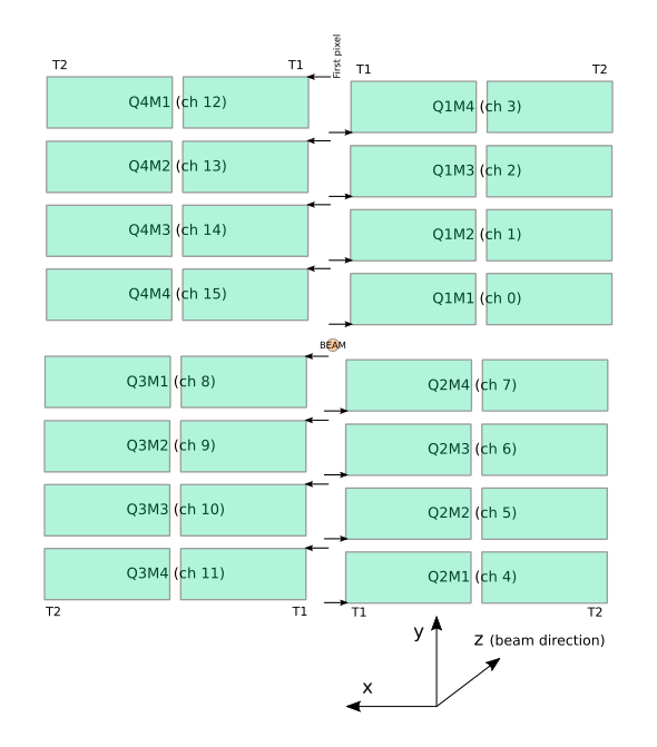
LPD-1M¶

LPD-1M consists of 16 supermodules of 256×256 pixels each. Each supermodule is further subdivided into 16 sensor tiles, which this geometry code can position independently.

The approximate layout of LPD-1M, in a front view (looking along the beam).¶

class karabo_data.geometry2.LPD_1MGeometry(modules, filename='No file')¶

Detector layout for LPD-1M

The coordinates used in this class are 3D (x, y, z), and represent metres.

You won’t normally instantiate this class directly: use one of the constructor class methods to create or load a geometry.

classmethod from_quad_positions(quad_pos, *, unit=0.001, asic_gap=None, panel_gap=None)¶

Generate an LPD-1M geometry from quadrant positions.

This produces an idealised geometry, assuming all modules are perfectly flat, aligned and equally spaced within their quadrant.

The quadrant positions refer to the corner of each quadrant where module 4, tile 16 is positioned. This is the corner of the last pixel as the data is stored. In the initial detector layout, the corner positions are for the top left corner of the quadrant, looking along the beam.

The origin of the coordinates is in the centre of the detector. Coordinates increase upwards and to the left (looking along the beam).

Parameters

quad_pos (list of 2-tuples) – (x, y) coordinates of the last corner (the one by module 4) of each quadrant.
unit (float, optional) – The conversion factor to put the coordinates into metres. The default 1e-3 means the numbers are in millimetres.
asic_gap (float, optional) – The gap between adjacent tiles/ASICs. The default is 4 pixels.
panel_gap (float, optional) – The gap between adjacent modules/panels. The default is 4 pixels.

classmethod from_h5_file_and_quad_positions(path, positions, unit=0.001)¶

Load an LPD-1M geometry from an XFEL HDF5 format geometry file

The quadrant positions are not stored in the file, and must be provided separately. By default, both the quadrant positions and the positions in the file are measured in millimetres; the unit parameter controls this.

The origin of the coordinates is in the centre of the detector. Coordinates increase upwards and to the left (looking along the beam).

This version of the code only handles x and y translation, as this is all that is recorded in the initial LPD geometry file.

Parameters

path (str) – Path of an EuXFEL format (HDF5) geometry file for LPD.
positions (list of 2-tuples) – (x, y) coordinates of the last corner (the one by module 4) of each quadrant.
unit (float, optional) – The conversion factor to put the coordinates into metres. The default 1e-3 means the numbers are in millimetres.

classmethod from_crystfel_geom(filename)¶

Read a CrystFEL format (.geom) geometry file.

Returns a new geometry object.

write_crystfel_geom(filename, *, data_path='/entry_1/instrument_1/detector_1/data', mask_path=None, dims=('frame', 'modno', 'ss', 'fs'), adu_per_ev=None, clen=None, photon_energy=None)¶

Write this geometry to a CrystFEL format (.geom) geometry file.

Parameters

filename (str) – Filename of the geometry file to write.
data_path (str) – Path to the group that contains the data array in the hdf5 file. Default: '/entry_1/instrument_1/detector_1/data'.
mask_path (str) – Path to the group that contains the mask array in the hdf5 file.
dims (tuple) – Dimensions of the data. Extra dimensions, except for the defaults, should be added by their index, e.g. (‘frame’, ‘modno’, 0, ‘ss’, ‘fs’) for raw data. Default: ('frame', 'modno', 'ss', 'fs'). Note: the dimensions must contain frame, ss, fs.
adu_per_ev (float) – ADU (analog digital units) per electron volt for the considered detector.
clen (float) – Distance between sample and detector in meters
photon_energy (float) – Beam wave length in eV

get_pixel_positions(centre=True)¶

Get the physical coordinates of each pixel in the detector

The output is an array with shape like the data, with an extra dimension of length 3 to hold (x, y, z) coordinates. Coordinates are in metres.

If centre=True, the coordinates are calculated for the centre of each pixel. If not, the coordinates are for the first corner of the pixel (the one nearest the [0, 0] corner of the tile in data space).

to_distortion_array(allow_negative_xy=False)¶

Return distortion matrix for LPD detector, suitable for pyFAI.

Parameters

allow_negative_xy (bool) – If False (default), shift the origin so no x or y coordinates are negative. If True, the origin is the detector centre.

Returns

out – Array of float 32 with shape (4096, 256, 4, 3). The dimensions mean:

4096 = 16 modules * 256 pixels (slow scan axis)
256 pixels (fast scan axis)
4 corners of each pixel
3 numbers for z, y, x

Return type

ndarray

plot_data_fast(data, *, axis_units='px', frontview=True, ax=None, figsize=None, colorbar=True, **kwargs)¶

Plot data from the detector using this geometry.

This approximates the geometry to align all pixels to a 2D grid.

Returns a matplotlib axes object.

Parameters

data (ndarray) – Should have exactly 3 dimensions, for the modules, then the slow scan and fast scan pixel dimensions.
axis_units (str) – Show the detector scale in pixels (‘px’) or metres (‘m’).
frontview (bool) – If True (the default), x increases to the left, as if you were looking along the beam. False gives a ‘looking into the beam’ view.
ax (~matplotlib.axes.Axes object, optional) – Axes that will be used to draw the image. If None is given (default) a new axes object will be created.
figsize (tuple) – Size of the figure (width, height) in inches to be drawn (default: (10, 10))
colorbar (bool, dict) – Draw colobar with default values (if boolean is given). Colorbar appearance can be controlled by passing a dictionary of properties.
kwargs – Additional keyword arguments passed to ~matplotlib.imshow

position_modules_fast(data, out=None)¶

Assemble data from this detector according to where the pixels are.

This approximates the geometry to align all pixels to a 2D grid.

Parameters

data (ndarray) – The last three dimensions should match the modules, then the slow scan and fast scan pixel dimensions.
out (ndarray, optional) – An output array to assemble the image into. By default, a new array is allocated. Use output_array_for_position_fast() to create a suitable array. If an array is passed in, it must match the dtype of the data and the shape of the array that would have been allocated. Parts of the array not covered by detector tiles are not overwritten. In general, you can reuse an output array if you are assembling similar pulses or pulse trains with the same geometry.

Returns

out (ndarray) – Array with one dimension fewer than the input. The last two dimensions represent pixel y and x in the detector space.
centre (ndarray) – (y, x) pixel location of the detector centre in this geometry.

output_array_for_position_fast(extra_shape=(), dtype=<class 'numpy.float32'>)¶

Make an empty output array to use with position_modules_fast

You can speed up assembling images by reusing the same output array: call this once, and then pass the array as the out= parameter to position_modules_fast(). By default, it allocates a new array on each call, which can be slow.

Parameters

extra_shape (tuple, optional) – By default, a 2D output array is generated, to assemble a single detector image. If you are assembling multiple pulses at once, pass extra_shape=(nframes,) to get a 3D output array.
dtype (optional (Default: np.float32)) –

inspect(axis_units='px', frontview=True)¶

Plot the 2D layout of this detector geometry.

Returns a matplotlib Axes object.

Parameters

axis_units (str) – Show the detector scale in pixels (‘px’) or metres (‘m’).
frontview (bool) – If True (the default), x increases to the left, as if you were looking along the beam. False gives a ‘looking into the beam’ view.

data_coords_to_positions(module_no, slow_scan, fast_scan)¶

Convert data array coordinates to physical positions

Data array coordinates are how you might refer to a pixel in an array of detector data: module number, and indices in the slow-scan and fast-scan directions. But coordinates in the two pixel dimensions aren’t necessarily integers, e.g. if they refer to the centre of a peak.

module_no, fast_scan and slow_scan should all be numpy arrays of the same shape. module_no should hold integers, starting from 0, so 0: Q1M1, 1: Q1M2, etc.

slow_scan and fast_scan describe positions within that module. They may hold floats for sub-pixel positions. In both, 0.5 is the centre of the first pixel.

Returns an array of similar shape with an extra dimension of length 3, for (x, y, z) coordinates in metres.

DSSC-1M¶

DSSC-1M consists of 16 modules of 128×512 pixels each. Each module is further subdivided into 2 sensor tiles, which this geometry code can position independently.

The approximate layout of DSSC-1M, in a front view (looking along the beam).¶

The pixels in each DSSC module are tesselating hexagons. This geometry code does not yet handle this: it treats the pixels as rectangles to simplify processing. This is adequate for previewing detector images, but some pixels will be approximately half a pixel width from their true position.

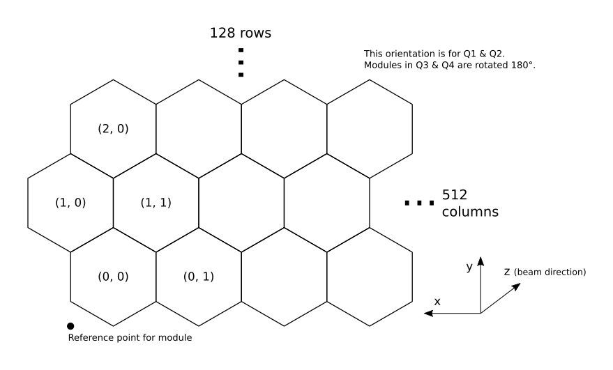
Detail of hexagonal pixels in the corner of one DSSC module.¶

class karabo_data.geometry2.DSSC_1MGeometry(modules, filename='No file')¶

Detector layout for DSSC-1M

The coordinates used in this class are 3D (x, y, z), and represent metres.

You won’t normally instantiate this class directly: use one of the constructor class methods to create or load a geometry.

classmethod from_h5_file_and_quad_positions(path, positions, unit=0.001)¶

Load a DSSC geometry from an XFEL HDF5 format geometry file

The quadrant positions are not stored in the file, and must be provided separately. The position given should refer to the bottom right (looking along the beam) corner of the quadrant.

By default, both the quadrant positions and the positions in the file are measured in millimetres; the unit parameter controls this.

The origin of the coordinates is in the centre of the detector. Coordinates increase upwards and to the left (looking along the beam).

This version of the code only handles x and y translation, as this is all that is recorded in the initial LPD geometry file.

Parameters

path (str) – Path of an EuXFEL format (HDF5) geometry file for DSSC.
positions (list of 2-tuples) – (x, y) coordinates of the last corner (the one by module 4) of each quadrant.
unit (float, optional) – The conversion factor to put the coordinates into metres. The default 1e-3 means the numbers are in millimetres.

get_pixel_positions(centre=True)¶

Get the physical coordinates of each pixel in the detector

The output is an array with shape like the data, with an extra dimension of length 3 to hold (x, y, z) coordinates. Coordinates are in metres.

If centre=True, the coordinates are calculated for the centre of each pixel. If not, the coordinates are for the first corner of the pixel (the one nearest the [0, 0] corner of the tile in data space).

to_distortion_array(allow_negative_xy=False)¶

Return distortion matrix for DSSC detector, suitable for pyFAI.

Parameters

allow_negative_xy (bool) – If False (default), shift the origin so no x or y coordinates are negative. If True, the origin is the detector centre.

Returns

out – Array of float 32 with shape (2048, 512, 6, 3). The dimensions mean:

2048 = 16 modules * 128 pixels (slow scan axis)
512 pixels (fast scan axis)
6 corners of each pixel
3 numbers for z, y, x

Return type

ndarray

plot_data_fast(data, *, axis_units='px', frontview=True, ax=None, figsize=None, colorbar=False, **kwargs)¶

Plot data from the detector using this geometry.

This approximates the geometry to align all pixels to a 2D grid.

Returns a matplotlib axes object.

Parameters

data (ndarray) – Should have exactly 3 dimensions, for the modules, then the slow scan and fast scan pixel dimensions.
axis_units (str) – Show the detector scale in pixels (‘px’) or metres (‘m’).
frontview (bool) – If True (the default), x increases to the left, as if you were looking along the beam. False gives a ‘looking into the beam’ view.
ax (~matplotlib.axes.Axes object, optional) – Axes that will be used to draw the image. If None is given (default) a new axes object will be created.
figsize (tuple) – Size of the figure (width, height) in inches to be drawn (default: (10, 10))
colorbar (bool, dict) – Draw colobar with default values (if boolean is given). Colorbar appearance can be controlled by passing a dictionary of properties.
kwargs – Additional keyword arguments passed to ~matplotlib.imshow

position_modules_fast(data, out=None)¶

Assemble data from this detector according to where the pixels are.

This approximates the geometry to align all pixels to a 2D grid.

Parameters

data (ndarray) – The last three dimensions should match the modules, then the slow scan and fast scan pixel dimensions.
out (ndarray, optional) – An output array to assemble the image into. By default, a new array is allocated. Use output_array_for_position_fast() to create a suitable array. If an array is passed in, it must match the dtype of the data and the shape of the array that would have been allocated. Parts of the array not covered by detector tiles are not overwritten. In general, you can reuse an output array if you are assembling similar pulses or pulse trains with the same geometry.

Returns

out (ndarray) – Array with one dimension fewer than the input. The last two dimensions represent pixel y and x in the detector space.
centre (ndarray) – (y, x) pixel location of the detector centre in this geometry.

output_array_for_position_fast(extra_shape=(), dtype=<class 'numpy.float32'>)¶

Make an empty output array to use with position_modules_fast

You can speed up assembling images by reusing the same output array: call this once, and then pass the array as the out= parameter to position_modules_fast(). By default, it allocates a new array on each call, which can be slow.

Parameters

extra_shape (tuple, optional) – By default, a 2D output array is generated, to assemble a single detector image. If you are assembling multiple pulses at once, pass extra_shape=(nframes,) to get a 3D output array.
dtype (optional (Default: np.float32)) –

inspect(axis_units='px', frontview=True)¶

Plot the 2D layout of this detector geometry.

Returns a matplotlib Axes object.

Parameters

axis_units (str) – Show the detector scale in pixels (‘px’) or metres (‘m’).
frontview (bool) – If True (the default), x increases to the left, as if you were looking along the beam. False gives a ‘looking into the beam’ view.